Open Colorimeter Plus: Implementing the dual light sensor design

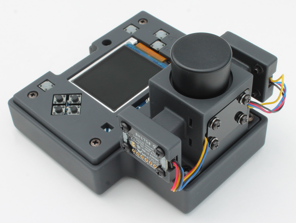
In this post we provide an update on the Open Colorimeter Plus design. The Open Colorimeter Plus uses a right-angle (R/A) or 90° measurement sensor as described in previous posts. This design extends the types of measurements the Open Colorimeter can perform to include fluorescence and light-scattering e.g. turbidity. Recently we added a second light sensor positioned at 180° i.e. facing the LED board. This 180° sensor measures the output light intensity from the LED which can then be used in different experimental approaches such as normalizing data to the applied light-intensity.

Open Colorimeter Plus with dual light sensors

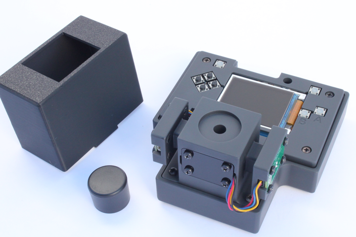
The 180° sensor we are using is the Adafruit BH1750 Light Sensor - STEMMA QT/Qwiic. This is an inexpensive $4.50 light sensor with STEMMA connectors so it can be easily connected to the Open Colorimeter Plus as shown below.

Implementing the 180° sensor

The interface to the BH1750 light sensor was added to the CiruitPython firmware using the Adafruit_CircuitPython_BH1750 library. This library is part of Adafruit's CircuitPython library bundle. The latest releases for the CircuitPython library bundle can be downloaded from here.

Adafruit BH1750 Ambient Light Sensor

This is the BH1750 16-bit Ambient Light sensor from Rohm. Because of how important it is to humans an most other living things, sensing the amount of light in an environment is a common place to get started when learning to work with microcontrollers and sensors. Should we turn up the brightness of…

Adafruit Learning SystemBryan Siepert

Testing the dual light sensor design

In this initial testing, we used different white light LED boards and measured baseline light intensity and the scattered light intensity from a single 100 NTU turbidity standard. The goals of these tests were to:

• Confirm that the Open Colorimeter Plus can measure both light intensity at the 180° calibration sensor and light-scattering at the 90° measurement sensor
• Measure variations in baseline LED intensities between unique LED boards
• Determine the relationship between baseline LED light intensity measured by the 180° sensor and the scattered light intensity from the 100 NTU sample measured by the 90° sensor
• Use the relationship, discovered above, to create a procedure which compensates for the differences in baseline LED intensity - enabling normalization of measured values.

Procedure

• Mount a white light LED onto the Open Colorimeter Plus
• Place a "blank" cuvette with water into the instrument
• Record the baseline LED intensity using the 180° sensor
• Place a 100 NTU standard into the instrument
• Record light scattered light intensity through the sample using the 90° sensor
• Repeat with a different white light LEDs

Results

Figure 1 below shows the scattered light intensity measured using the 100 NTU sample (90° light sensor) vs. baseline LED intensity (180° light sensor).

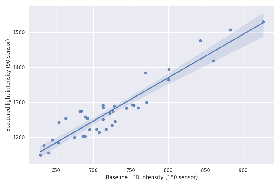
There is a clear linear relationship between scattered light intensity, $I_\mathrm{s}$, and the baseline LED light intensity, $I_\mathrm{b}$, such that

$$ I_\mathrm{s} = \mathrm{slope} \times I_\mathrm{b} + \mathrm{offset}.$$

The slope and offset of the linear relationship can be estimated using a linear least squares regression. Next, a normalization procedure for scattered light intensity $I_\mathrm{s}$ can be developed using the slope of the linear relationship.

In order to do this we first pick a reference baseline LED light intensity $I_\mathrm{b,ref}$. We then adjust our measured intensity $I_\mathrm{s}$ to the value it would have $I_\mathrm{s,nrm}$ if the baseline LED light intensity was equal to the reference value $I_\mathrm{b,ref}$. This is done as follows

$$I_\mathrm{s,nrm} = I_\mathrm{s} + \mathrm{slope} \times \left( I_\mathrm{b,ref} - I_\mathrm{b} \right).$$

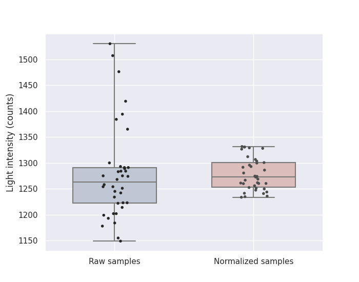
Next we applied the normalization above to the data collected for a single 100 NTU sample with different white light LEDs. As you can clearly see in Figure 2 the normalization procedure greatly reduces the variance of the measured values due to the differing baseline LED light intensities.

The two data plots above were prepared using Matplotlib and Seaborn python libraries.

This was a preliminary experiment to demonstrate the new dual light sensor feature of the Open Colorimeter Plus. Below are some of our next development steps!

• Designing an additional through-hole LED board option
• Modifying the sample holder design to bring sensors and LED closer to the sample
• Updating and releasing the open source firmware to include measurements for the Open Colorimeter Plus

Open Colorimeter Plus Form

Hello! We are currently completing development of the Open Colorimeter Plus. This is an expanded version of the Open Colorimeter that expands measurements to include fluorometry and turbidity (light-scattering). We expect to release this open hardware science instrument in Fall 2023 but you can sign…

Google Docs