Protein Quantification with the UV Open Colorimeter
In this tutorial we are using the new UV Open Colorimeter for A280 protein quantification measurements using a UV sensor and 270-280 nm UV LED
Background
Protein concentration is an extremely useful and routine measurement in science with a wide variety of applications in biochemistry, molecular biology, environmental and biomedical research. Common methods for measuring proteins are colorimetric assays such as the Bradfords method and spectrophotometric analyses such as absorbance at 280 nm (A280). This latter test is fairly straightforward requiring no extra reagents or incubation time and is the focus of this tutorial.
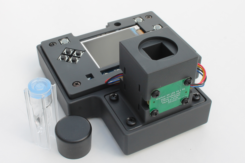
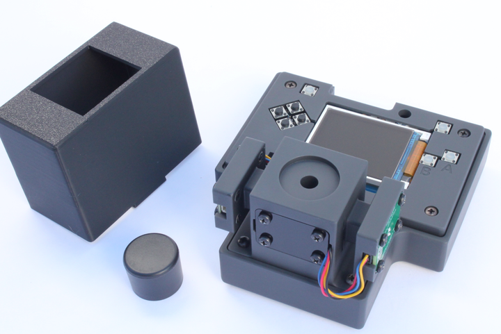
A280 measurements require a specific instrument, usually a UV/Vis spectrophotometer. However, A280 measurements can also be carried out with the new UV Open Colorimeter. This instrument uses the AS7331 UV Sensor Board in combination with a UV LED. We currently have two LEDs in the 270-280nm range that work for this purpose - 275nm and 278 nm. You can learn more about the LEDs and UV Sensor in the Open Colorimeter Product Guide.
Molar extinction coefficient (ε) is a measure of how strongly a substance absorbs light at a particular wavelength, and is usually represented by the unit M-1 cm-1. The ε of a specific protein at 280 nm depends almost exclusively on the number of UV-light absorbing aromatic residues - particularly tryptophan (Trp) and tyrosine (Tyr). ε of a protein can be predicted from the sequence of amino acids. UV absorbance of aromatic amino acids is shown in the graph below from Hammod et. al (2014). Note the absorbance peak at around 280 nm for Trp and Tyr.
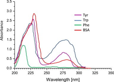
BSA (bovine serum albumin) is a widely used standard for protein quantification and is commonly available from most scientific reagent suppliers. In the above graph, we can also see the absorbance profile of BSA.
From the literature, we know that the molar extinction coefficient, ε, for BSA at 280 nm (ε280 ) is 43,824 M-1 cm-1. Knowing the molar extinction coefficient, you can predict the absorbance values when Beer's Law holds true i.e. the relationship between absorbance and concentration is linear. We know from the literature that BSA has a linear relationship between concentration range of 0-2 mg/mL A280. Using this information we can determine the protein concentration of unknown samples.
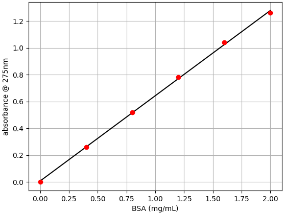
In this experiment, we are using the new UV Open Colorimeter to prepare a 0-2 mg/mL linear BSA calibration which will be saved onto the instrument for later protein quantification measurements. In the second part we calculate ε of BSA from our collected data and compare this to the known value. This serves the purpose of double-checking that our UV Open Colorimeter instrument and methods are all working as expected.
Materials
- UV Open Colorimeter with 275 nm UV LED
- 2 mg/mL BSA standard
- For this tutorial we used the albumin standard from GenDEPOT which cost $36 for 5 x 1mL tubes of 2 mg/mL BSA. However, any BSA standard would work
- 6 x UV transparent micro cuvettes - 15 mm center height.
- With the Open Colorimeter these cuvettes have a minimum fill volume of 0.4 mL
- 6 x 1.5 mL microcentrifuge tubes
- 0.2-1.0 mL adjustable micropipettes
- Distilled water or buffer
Part 1) Prepare BSA solutions for calibration
Use the table below to prepare a 6-point BSA dilution series. In this example we used 1.5 mL microcentrifuge tubes to make the dilutions of BSA.
| BSA Conc. |
BSA Standard | distilled H₂O |
|---|---|---|
| 0.0 mg/mL | 500 µL | 0 µL |
| 0.4 mg/mL | 400 µL | 100 µL |
| 0.8 mg/mL | 300 µL | 200 µL |
| 1.2 mg/mL | 200 µL | 300 µL |
| 1.6 mg/mL | 100 µL | 400 µL |
| 2.0 mg/mL | 0 µL | 500 µL |
Part 2) Measure UV Absorbance of BSA
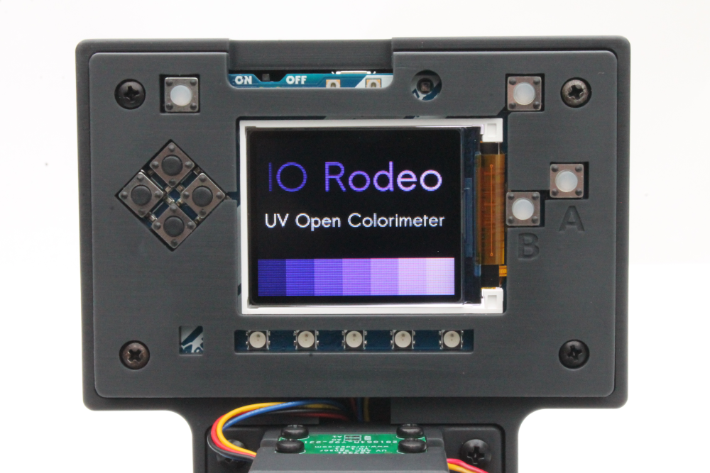
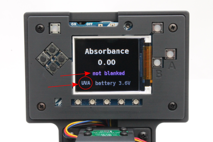
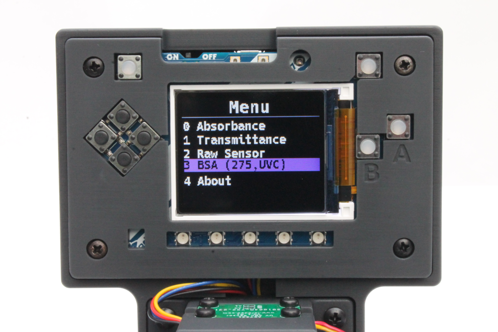
- Switch on the UV Open Colorimeter. After the splash screen, the first screen is the default Absorbance screen as shown below. You can see that i) the UVA channel is selected and ii) the instrument is "not blanked" so these are the next steps
- Select UV-C Channel: In the 4-button Menu Navigation, the far-left button is used to toggle between UV-A, UV-B and UV-C channels. Use this to select the UV-C channel
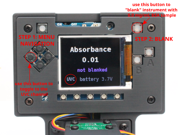
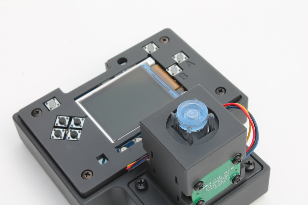
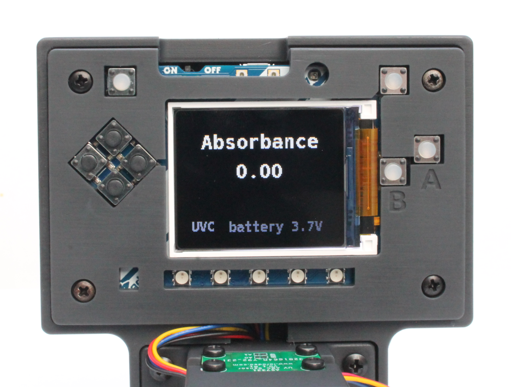
- Blanking: Next, transfer the 0.0 BSA sample into a cuvette and blank the Open Colorimeter using the top right "blank" button as shown in the image above. After these two steps the Open Colorimeter screen should appear like the image below and is ready for absorbance measurements.
- Measurements: Transfer the 0.4 mg/mL sample into a microcuvette and record the absorbance value. Repeat for samples: 0.8, 1.2, 1.6 and 2.0 mg/mL. An example screen is shown below. Record your values.

Part 3) Create a BSA calibration method for the Open Colorimeter
In this step we will use the oc-calibration-app to plot the data collected and export a calibration file for the Open Colorimeter. We have previously shared similar steps in the Part 2 of the Bradfords assay tutorial.
i) Save formatted data
For importing data into the oc-calibration app, it needs to be saved as a .csv file. A CSV file can be easily generated using a spreadsheet application or a text editor. This should be a plain text file with two columns of data separated by commas. The first column of data should consist of the BSA concentration. The second column of data should consist of the absorbance measurements. An example .csv file with BSA absorbance data collected in this tutorial is attached below.
ii) Using the oc-calibration-app
Follow the instructions in this tutorial to import and plot your data. Once you have everything set, download the .json calibration data.
 William Dickson
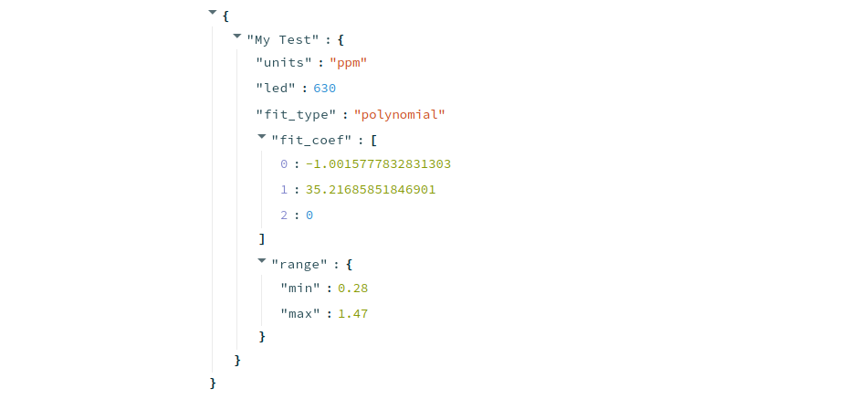
iii) Edit calibrations.json
Once you have downloaded the .JSON file from the oc-calibration-app, edit the calibrations.json file on the PyBadge to include the new BSA calibration data. Instructions on how to access and edit this file are in the tutorial "Customizing configuration and calibration files".
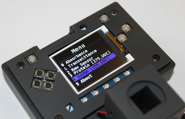
When you restart the Open Colorimeter the new calibration will show up as an option in the Menu as shown below.
iv) Using the saved BSA calibration for protein quantification
This method can now be used whenever you need to measure protein concentration. Select the saved method from the Menu and it will automatically select the UV-C channel and return measurements in mg/mL.
Part 4) Experimental determination of BSA molar extinction coefficient
According to Beer's law:
- A = εbc
- A is the absorbance
- ε is the molar extinction coefficient
- b is the path length of the cuvette
- c is the concentration
ε can be obtained by calculating the slope of the absorbance vs. concentration plot. Previously we have described how to experimentally measure ε using food dye as an example.
In the next steps we describe how to calculate ε of BSA from our UV absorbance data collected above and compare this to the known ε280 value of 43,824 M-1 cm-1:
- Step 1: Convert BSA concentration from mg/mL to Molar concentration.
- BSA has a molecular weight of 66,463. Dividing mg/mL concentration by 66,463 = M concentration
- Step 2: Plot absorbance versus M concentration. Find the slope of the plot.
- The slope is the ε275 of BSA. In the data from this experiment, ε275 is 42,251 cm-1M-1
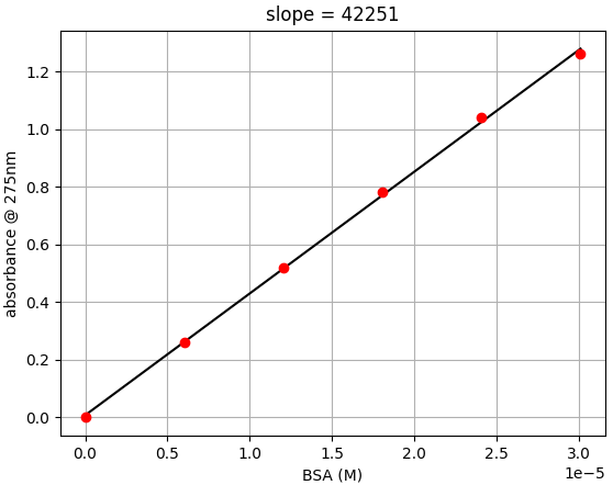
- Step 3: Calculate the % experimental difference
- In this example we see there is only a 3.6% different than the expected value of 43,824 cm-1M-1
Comments ()